What I worked on This Week
Data Reduction Pipeline
I am very excited to say that as of this week, I believe my data reduction pipeline is polished and complete. I have resisted the urge to go back and clean up my old code and instead have opted to test edge cases and unique events to make sure that it holds up to sizable stress. So far it has done quite well and it looks as though I can lay the beast to rest, focusing now on the photometry pipeline (yayyyyy! progresssss!)
Photometry pipeline creation
I began this week by reviewing my code from 337 which extracted photometry from our cluster images. It took a bit for me to fully refresh my memory as to what the code was really doing, but because of my stellar commenting the process was extremely smooth :). For this project I began by running my photometry code from some of the old colab notebooks. While it seemed to work well for most images, there were a few that returned photometry tables that were completely off. I’m still not sure why they weren’t working as expected, but I have a few ideas that I have detailed below. The first was the fact that I have not been padding my images before alignment. I’m pretty sure the lack of alignment is leading to some stars getting cut off which is leading to some strange photometric values.
Image Padding
To fix this I have been padding images by 25 pixels, which in general has been enough. This value is the constant number of pixels we used last year for padding, so I simply ported it over. I’m not sure the best way to create a dynamic value here, as it will be based on the amount the telescope shifts each night. The downside of increasing this value drastically would be an increased runtime for all of the following photometry functions. I think the way I’ll approach this for the rest of the semester is to include a default padding variable and check to see if any centroid returns a higher value. If it does then I can just add 25 pixels plus the centroiding value which should be enough protect against any edge cases.
Next Steps
For the major photometry pipeline, all I need to do is finalize the edge cases so that the photometry tables turn out accurately across nights. This shouldn’t be too much work, as the code seemed to run smoothly last year and from what testing I have done, will continue to this semester as well. Other than that, I need to create a storage system to organize the photometry tables in a way where I can overwrite but also back them all up. This shouldn’t be too hard to implement, but it will take a bit of thought if I want to design it well. I would also quite like to have this code be generalizable for future projects if I can.
Results from Light Curve Exploration
Light curve preparation
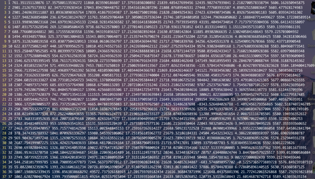
As discussed above, I created photometry tables using data from one night so far. The tables contained generally promising values, but there is a lot of fine tuning that I will want to do before finalizing the data. Below is a screenshot of some of the files where a couple erratic entries can be seen throughout. (Although I am not sure if any of those entries made it into this screenshot.) In addition, I want to fine tune some of the aperture and annulus values that went into these estimates. I am still using the values from last year and will refer to some of the in class discussions we had to choose better values later this week. So far I have been more focused on making sure the code and logic work as opposed to the actual input values for each function.
Centroiding and Cross-correlation
One set of errors that have kept popping up are concerning image alignment. For some reason, even though I am aligning all of my images to the same single fits file, they keep appearing off by slight amounts. When I blink through the aligned files on DS9, they appear to be off by the slightest of errors. I spent a lot of time this week looking into why this could be, and I think it has something to do with the centroiding function. From what I can tell, my cross correlation algorithm is working quite well, but the subpixel corrections are somehow off. I don’t know if it’s an x versus y coordinate confusion or just some bug in the code, but this coming week I think I’ll try substituting my own centroiding math from last semester in so that I can see if there is any change.
Next Steps
As discussed above, I want to search for optimal organization for all my data tables, find optimal input values for my apertures and annuli, and then eventually debug the inaccuracies in the centroiding code. It will also help to know at our OOC meeting tomorrow whether or not I am the only one with this sort of issue. If I am then maybe it has to do with the way in which my images are being accessed or input into the alignment code, or maybe I just need to pad a few pixels because of an even/odd pixel range error. Either way, the plan is to fix this by the code submission on Friday.
AAVSO Folding exercise
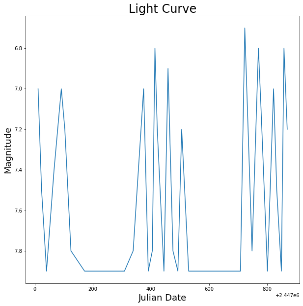
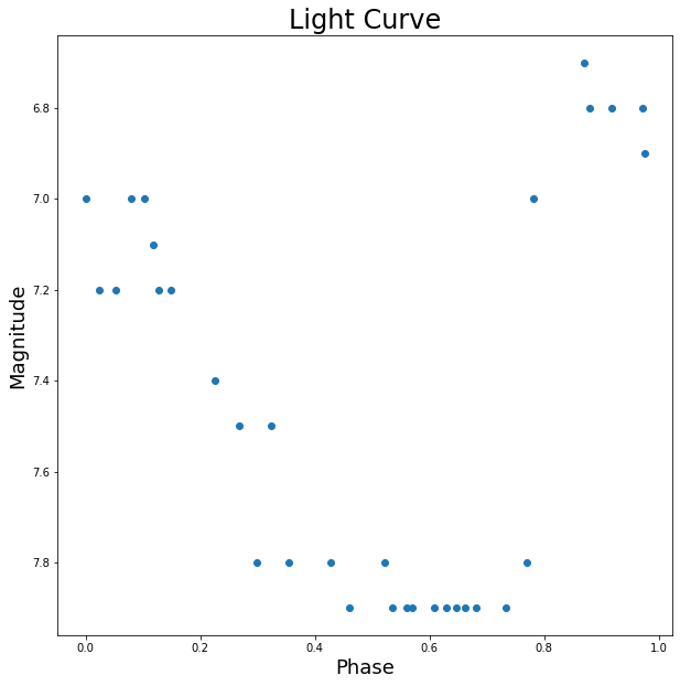
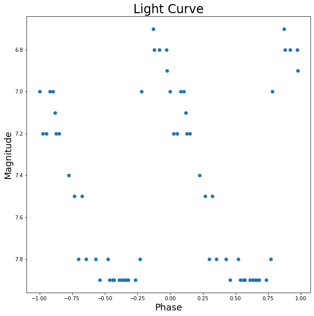
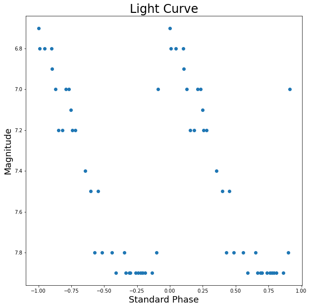
Above are the four graphics from the exercise which had us play with photometry data to generate some basic light curves. From the first graphic, we can see that there aren’t any clear trends in the data. It seems as though there is a somewhat periodic spiking for the days in which we have data, but there are not enough data points to be sure by eye. From the second graph, however, it seems here that the data could be fit well with a curve as the deviations are close to 0.2 magnitudes, which is within the defined error threshold. The third graph looks quite good and a curve could most likely be fit quite well to this data. The curves line up well around the connection point at x=0, so the choice of phase seesms to be quite good. Thus, the data could most likely be fit well with a curve. For the final graph, the maximum here does lie at phase 0, thus the epoch is pretty much correct. Most of the data can also be fit with a smooth curve meaning that most of our calculations incluced correct values.
Reading Notes
Overview
The paper mainly focuses on different mathematical and statistical techniques for analyzing light curves to determine periodicity. It focuses on a handful of the most powerful techniques that have been developed over a couple hundred years. Templeton then goes on to discuss the applications of such techniques, as well as their weaknesses and flaws. The paper ends with information on many other more advanced techniques and information on where to read about them in quite a bit more depth. I will mention a few of what I believe to be the most important sections below.
Fourier Transform
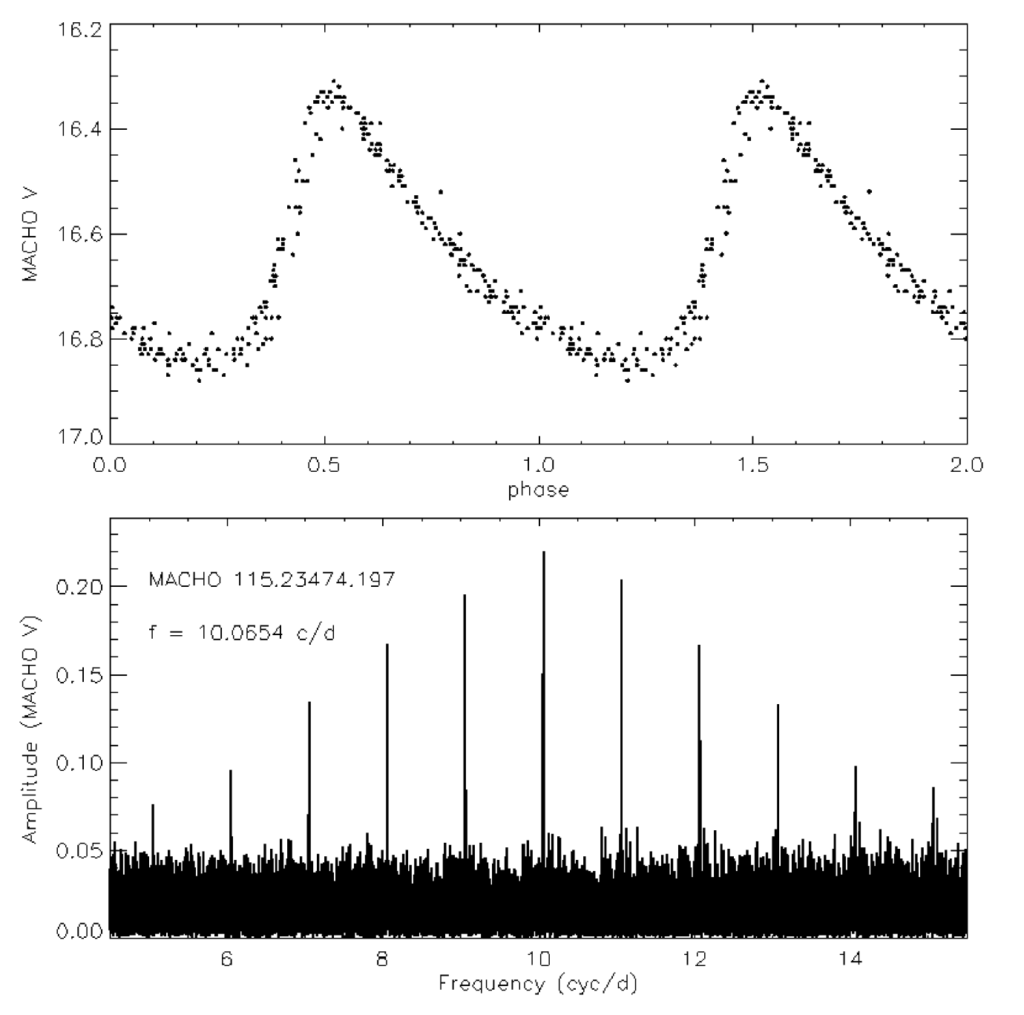
Fourier analysis is the technique of repeatedly integrating a continuous or discrete function for a range of given frequencies. From an analysis of the maxima of the integrated values, we can determine the most prevalent frequencies underlying the original continuous or discrete function. This method is incredibly powerful and has applications in almost every field. The Fourier Transform, however, is limited in the range of frequencies it can accurately obtain when examining time series data. It is also limited by the noise of the data and small periods are often overshadowed by relatively minimal amounts of noise. The paper then talked quite a bit about the applications of Fourier Analysis, specifically with regards to the Fast Fourier Transform, which runs in nlogn time, but requires some sacrifices in the sampling process that reduces its usefulness in our application. The image below shows a time series light curve on the top, plotted with phase on the x axis and vband magnitude on the y. The bottom graph is a Forier transform of this data with the “picket fence”-like peaks mentioned in the reading. The distribution of frequencies below the peaks also shows the transform’s weakness when it comes to noisy data.
Autocorrelation
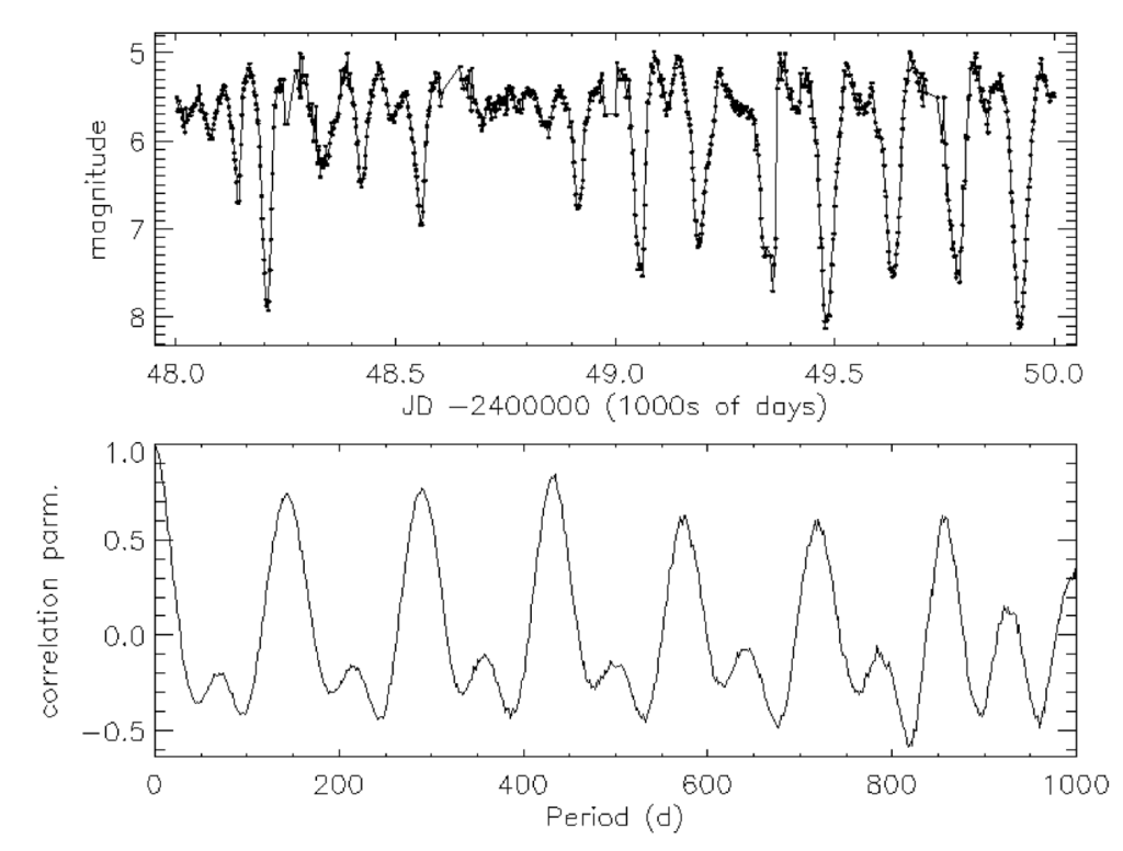
Templeton then discusses the autocorrelation technique, which, for its simplicity, is very powerful. The autocorrelation method simply posits that for a periodic function with period t, the values for any x and x+t will be very similar and thus highly correlated. In the same vein, for a random value of t, the two values at x and x+t will be very loosely correlated and thus not similar. By repeating this test for a large range of t values, we are able to determine strong candidates for possible periods and thereby frequencies within the data. The image below shows very detailed light curves at the top without an extremely clearly discernible period. The bottom graph shows the incredibly clear periodicity brought out through use of the autocorrelation method.
Paper Descriptions
Star Cluster Formation in Cosmological Simulations. I. Properties of Young Clusters by Hui et al. 2017
This paper uses simulations to present star clusters as locations of star formation. By calculating initial momentum and gas ratios, they are able to use IMF models to simulate the evolution of star clusters over large time scales. While the methods will not directly apply to our project, the physics discussed in this paper has already helped me understand a bit more about how the initial mass function correlates to the present day mass function and to what we will be observing in this course.
Mind Your Ps and Qs: The Interrelation between Period (P) and Mass-ratio (Q) Distributions of Binary Stars by Maxwell et al. 2017
This paper is in line with some of the conversations we have had about accounting for multiplicity in our measurements. In this paper they use a number of statistical methods to analyze previous observations with the goal of developing a better understanding of how multiplicity affects measurements. They produce a probability density function that could at least be interesting to dive into, even if it doesn’t directly influence the direction of our project. Overall this will be helpful in estimating possible error.
The evolution of CNO isotopes: a new window on cosmic star formation history and the stellar IMF in the age of ALMA by Romano et al. 2017
Finally, this paper is a bit more selfish. I saw there was a paper that talked about IMFs, CNO, and ALMA all in one go and I couldn’t help myself. In this paper they use chemical models to track gaseous flow in the ISM to constrain different IMFs. ALMA is positioned at the perfect wavelength range to observe a range of semi-heavy metals (3C, 15N, 17O and 18O, along with 12C, 14N as included in the paper) the abundance of which should not be greatly affected by recent star growth and eventual death.