Image Reduction
Update from the Week
This past week I focused on finishing my data reduction code and I think it’s currently in a really good place! I pulled the biases and darks from the iTelescope WTP server and ran them through the reduction process. (Technically reducing the bias is just for show because the data is skewed with what appears to be a linear offset, but the master bias will most likely be useful in the future for estimating read noise and other yet-to-be-discussed applications.) I combined three sets of darks at one, two, and three minute exposure times to create master darks. These master darks cannot be rescaled, however, as they are not bias corrected so we are stuck with their current exposure times.
The flats turned out to be a bit more confusing, the why of which I detailed extensively in my last blog post. In short, the flats have a range of exposure times and come already bias subtracted. After speaking with Connor, I was advised to not dark subtract my raw flats and instead just rescale and normalize them accordingly. Thus, I scaled the bias-subtracted flats to a one second exposure time and then median combined them into a single image. I then divided through by that image’s median to effectively normalize the final master flat. I generalized the code to repeat for any number of included bands, and voila! master flats were born.
The next step I tackled was the actual science data reduction. While we already had some code for this, I needed a much more generalized version that could be used for data taken over a range of nights. I ended up rewriting most of my code from last semester for this step, as I just know a bit more python now and can write slightly better code. My code now sorts the raw data and copies the raw images to be processed in the correct way necessary for this class (i.e. without bias subtracting and with un-bias-subtracted darks). I also wrote the code such that it is entirely backwards compatible, so if we want to at any point go back to bias subtracting things, only one function input needs to be changed and we’re right back to the good ol’ days.

Shift.py
How do the functions work?
• Centroiding — The centroiding function uses fascinating pixel math to determine the geometric center of a bright group of pixels. It uses a modified gradient descent calculation in two dimensions to find the “peak” pixel range. It is accurate enough, however, that it returns a sub-pixel measurement making it a very accurate method for determining the appropriate shifts. It takes two images and a general region within them and returns a set of offsets between the two.
• Cross-Correlation — The cross_image function uses the cross correlation of the two images to find a peak pixel that is used to determine offsets. This method employs the Fast Fourier Transform (FFT) algorithm which turns each image into a frequency space image that is much more efficient to cross correlate. While the upside compared to the centroiding function is efficiency, this method only returns a pixel value and not a sub-pixel offset, making it slightly less exact. Implemented here, however, it tries to use the centroiding function once it has already narrowed down the center region, thereby combining the two into a best performance scenario. It also takes two images and a general region within them and returns a set of offsets between the two.
• Shift-image — The shift image function simply runs an interpolation function that shifts the specified image by the offsets given in one or both of the previously described functions.
The Result
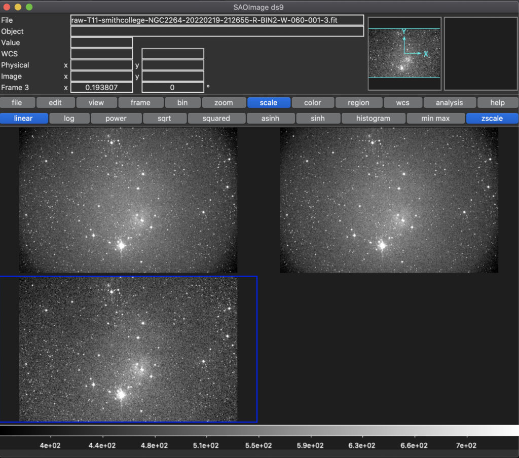
It took a bit to work out the kinks in implementing the code. Scipy’s interpolation function has a few quirks that make it finicky when dealing with nans. Other than that, the images processed really well and I now have a lot of aligned images. I would include them all here, but they are sort of redundant to include as they barely look different from before. As I have been working with data from a night with very low wind, my offsets are relatively minimal (only a few pixels for most of the images I looked at), which is to be expected.
Roadblocks
I actually don’t think there were very many major roadblocks this week! Hopefully that doesn’t mean I’m just saving them up to cash them in after break….
Next Steps
It looks like my next steps are going to be focused on extracting photometry (yay!). Now that all our images are sorted, reduced, and aligned, we can really begin focusing on how we want to process our data for the project. We’ve been discussing this step a bit as a group so I don’t think anything too challenging will come up with regards to the direction we’re going to take. I’ll probably look into Astrometry.net within the next week and start thinking about how differential photometry will work from a code standpoint, just so I’m prepared.
Differential Photometry
Differential photometry is a technique to recover relative magnitudes of stars within an image. We begin by extracting the photometries of all the stars within our cluster that we can resolve. If we were to examine the changes in these instrumental magnitudes over the course of the night, we might see some strange behaviors of the light curve fluxes. Most likely, these behaviors, such as dips and irregular patters, will occur for most if not all stars at the same time — this change could be due to a shift in seeing or some temporary cloud cover for example. No matter the cause, we can correct for the variation by assuming all the stars were affected in the same way, and thus looking only at the differences in magnitude of the stars across the night.
To do this however, we need to choose a baseline for our calibration. The baseline needs to be a single star that we know is not itself varying with respect to time. If we choose a variable star as our differential baseline, it will introduce clear error into the rest of our data. Assuming then we select our calibration star to be a star with low to no variability, we can determine relative fluxes and thus magnitudes compared to that single star. This technique should give us the relative photometry of all the stars in our cluster compared a single member. To determine the exact magnitudes, we would then only need one standard to correctly calibrate the magnitude of our single baseline star, thereby calibrating all the rest of our data for the semester.
CCD Activity
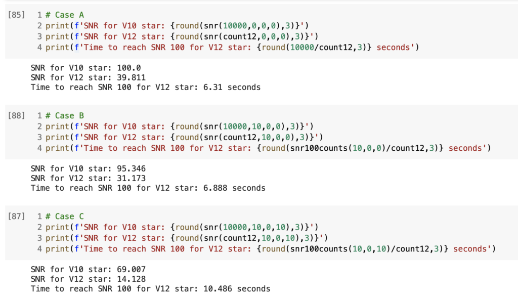
I completed the CCD activity using a jupyter notebook (ok fine it was colab im sorry that im sort of a degenerate 😊). I’ve included an image of the outputs for the three cases below, with my calculations printed after each of the three cells. Νωτ μι υς οφ φστρινγς, ιμ γεττινγ γοοδ ατ θις.

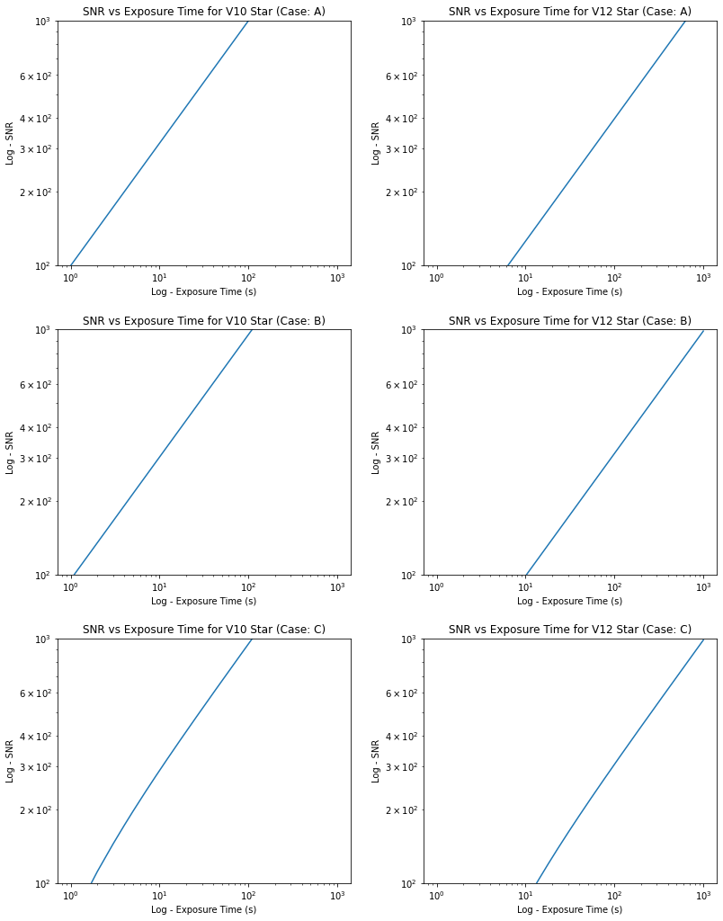
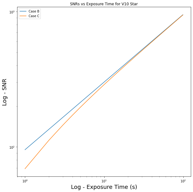
Below are the plots outlined in the slides. I’ve included the first six as a panel plot and then the last plot individually below. For the panel plot, I standardized the axis limits so that the slope and intercepts of the lines can be more easily compared. We can thus tell which lines are growing faster and which ones have a steeper offset.


And there’s week 4 done, wow it’s all just going so fast… Also N.B. you should click on the link above if you haven’t already. It’s in one of the paragraphs (I know the coloring doesn’t make it stand out too well). It’s from this really relevant and interesting thing I read on the interwebs I highly recommend clicking it. You should click it 🙂