Well, I guess we’re Finally Here (& reflections)
I can’t believe we made it to the last class. It’s been a long and wonderful road, the past few months. 🙂
- What was the most valuable part of the class for you?
– The most valuable parts of this class were the proposal writing and the weekly blogs. I am convinced that the proposal writing exercise will end up being extremely valuable if I continue my journey into any academic field, especially into physics or astronomy. The process has always seemed intimidating and unreachable, so I am so grateful that this course demystified the procedure. The weekly blogs were also essential to my ability to hold myself accountable throughout the course. Without these, I am sure I would have paid less attention to where I was with my weekly work and would have been generally less organized. - What would you have done differently
– I would have asked more questions. Although I understand a lot and learned so much from this year, there were always topics that I wanted to know more about or should have probed more deeply into. I’m so much better at this than I was though, so I’ll take my progress as a win. - What did you enjoy doing the most in the class? What did you not enjoy? How does this impact your future academic/industry career paths?
– I liked the quantitative elements and the pipeline building quite a bit. I still don’t know how I feel about experimental astro when compared to the theory, but everything I have heard has warned me to complete observational and applied research first, before going into theory. And I completely agree. This course has taught me so much of both, and I feel quite prepared for the next year and a half of research and coursework in these and related areas.
Final Results
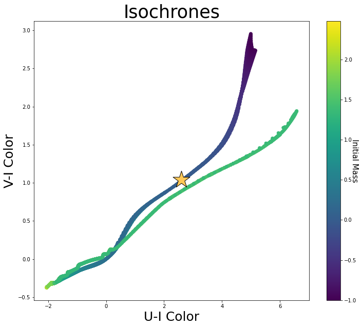
Our project turned out really well in my eyes. I am so proud of Meredith and Cat and the work we all were able to do. Below I have the isochrones we used with one of our stars plotted over top. The data is plotted in color – color space, where we eventually added one new point for each star we observed in all three bands. As our photometry got better and better over the last two weeks, we were able to improve the accuracy of star locations on this diagram, in this space. The more accurate their photometry became, the more accurately we would be able to connect them to well fitting isochrone.
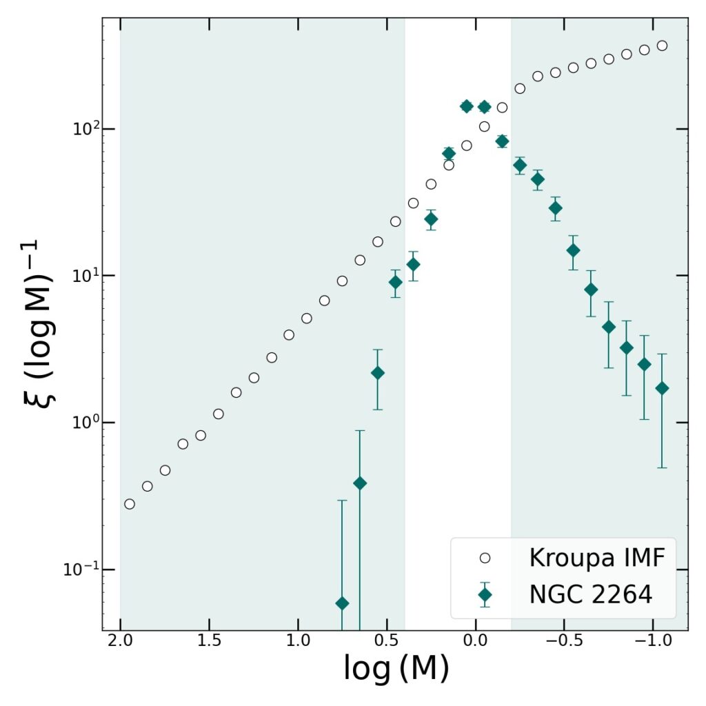
Below is our final IMF plot, which we have iterated and improved upon since last week. It more accurately fits the high mass end of the Kroupa IMF and the slopes are much closer than they were when we presented our work. We still have a ways to go in the low mass regime, some of which might be able to be improved by more detailed photometry techniques and a better reduction pipeline that would allow us to resolve dimmer stars in the cluster. If we had more time, it would be interesting to try to understand where T11’s limit really should be, and therefore how close we are with our data. Any significant gaps would point to possible improvements in our photometry and/or our stacking code.
Spectra lab
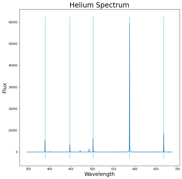
In this lab, we compared spectra from emission lamps to better understand and scale a separate spectrum of the sun. Below is a plot of a helium spectrum with five emission lines identified. We identified these emission lines by eye and were able to accurately determine the pixel values they landed on.
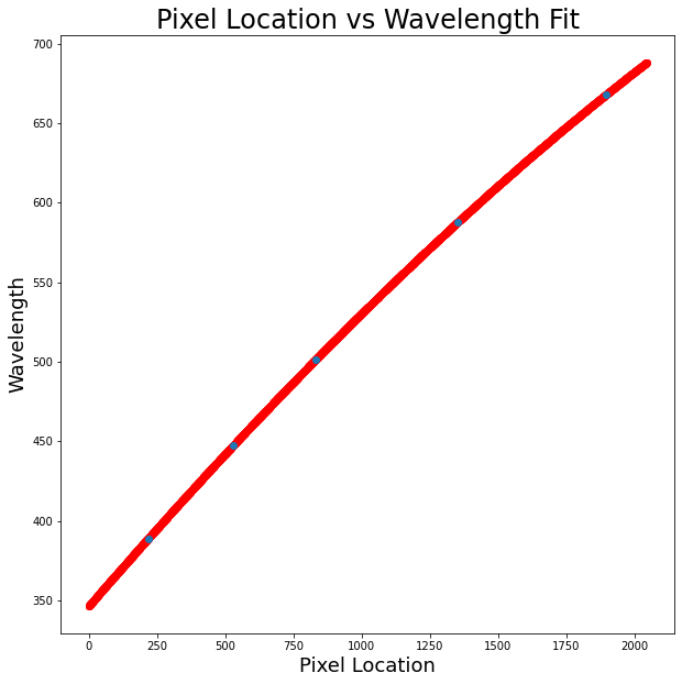
We then fit a third order polynomial to the pixel values to give us a continuous wavelength array.
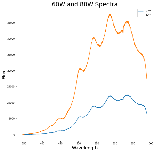
Below is a plot of reduced 60 Watt and 80 Watt bulb spectra. We will use these to create a response function.
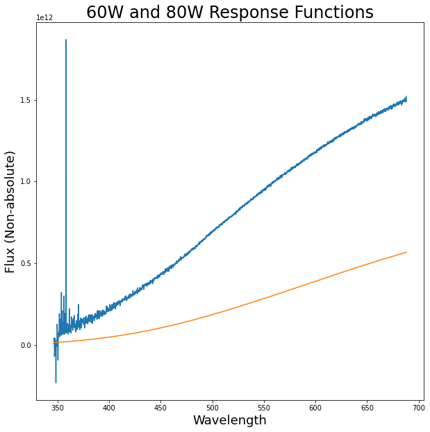
In blue, below, is the response function — generated using the 60 Watt bulb spectrum — divided by the 80 Watt bulb spectrum to see if we get a smooth curve. Below in orange is the planck model of the 60 Watt bulb for comparison. It has been artificially scaled to match the axes of the blue curve.
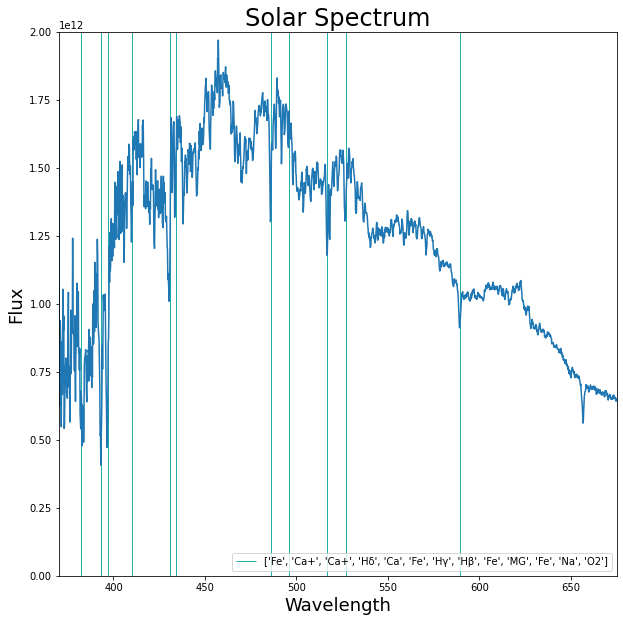
Using this response function, we were able to properly scale the solar spectrum and then overplot the Fraunhofer lines onto it. The elements causing the absorptions shown below are listed in the legend in a corresponding order.
Overall this was a really cool lab! I’m glad we had a chance to follow this process through and get a bit more insight into the handling of spectra.
Observation lab
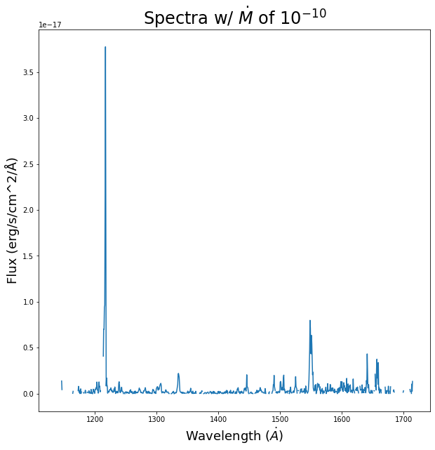
In this activity, we examined the spectrum of an actively accreting brown dwarf and scaled said spectrum to predict the spectra of different accreting objects we were hoping to observe. Below is the spectra of an object 60 pc away with a mass accretion rate of 10^-10 solar masses per year. In addition, all the negative values have been thrown out, which will bias the continuum, but for our sake when looking at lines, it will simplify the whole process.
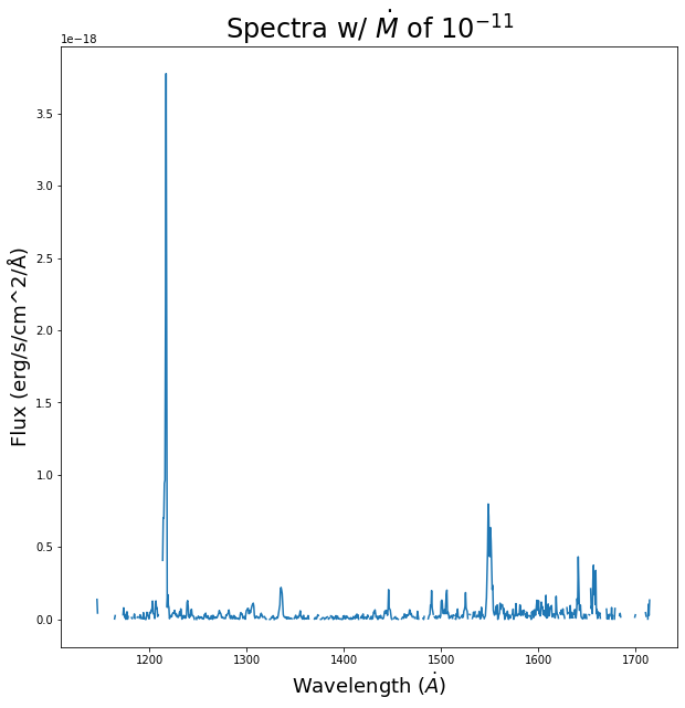
Below is the second spectra we wanted to generate, this time of an object 60 pc away with a mass accretion rate of 10^-11 solar masses per year. Similar to the plot above, all the negative values have been thrown out.
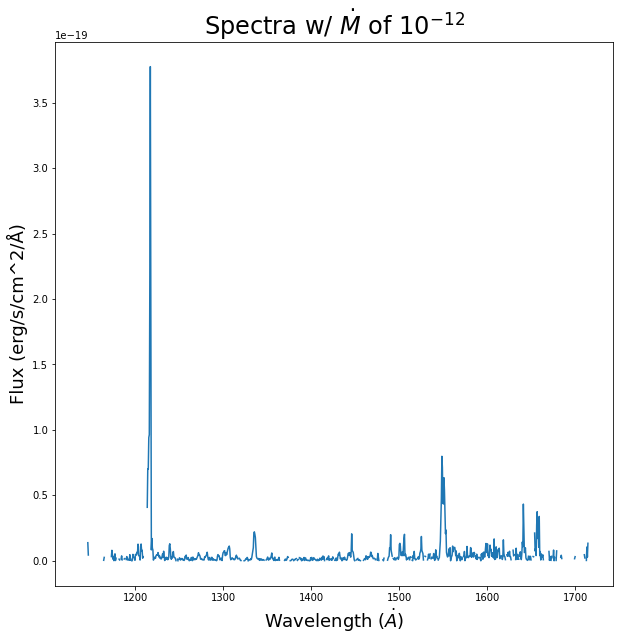
Finally, below is the third spectra we wanted to generate, this time of an object 60 pc away with a mass accretion rate of 10^-12 solar masses per year. Similar to the two plots above, all the negative values have been thrown out.
Unfortunately, over the last few days I have kept running into the same error with both calculators provided to us. I have followed all the instructions to a tee, but can’t seem to get anything out of them. I want to keep playing with this, so I’ll update this post if I can figure something out.

relevant Paper
For my paper, I chose one of the more recent MIST papers that incorporated quite a few new additions to the MESA toolkit. The paper is from 2015 and titled “Modules for Experiments in Stellar Astrophysics (MESA): Binaries, Pulsations, and Explosions.” The paper was quite long and dived pretty far into the inner workings of MESA, so I have included a few graphs below to help summarize some points I found interesting.
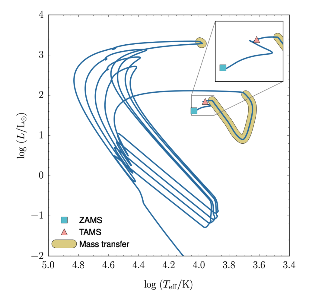
Although I read this paper to learn about isochrones and the best practices for more complex MIST models, I ended up learning a ton, and getting confused quite a bit by, some of the more complicated aspects of MESA. I’ve used MESA in the past to run simple models and create some straightforward evolutionary tracks, but the sorts of simulations they showed here blew me away entirely. Below is a binary system of a 2.5 M⊙ star transferring mass to a 1.4 M⊙ point mass with a discontinuous mass exchange and different stellar phases (ZAMS and TAMS) overplotted.
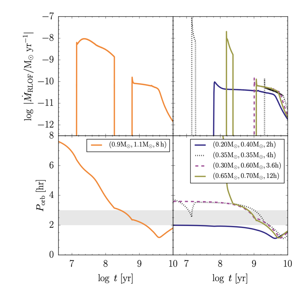
I had to include the plot below because I had no idea that anything like this was possible within MESA. I am going to have to revisit their software at some point in the next year because some of these simulations are unbelievable. These graphs show a Cataclysmic Variable actively accreting and while taking into account the effects of magnetic braking and gravitational wave radiation. I was entirely unaware that MESA could simulate anything this complex and am very interested in learning more about these assumptions. Parts of this paper go into quite a bit of detail on these techniques and I am looking forward to being a bit more free over the next few weeks to dive in somewhat deeper.
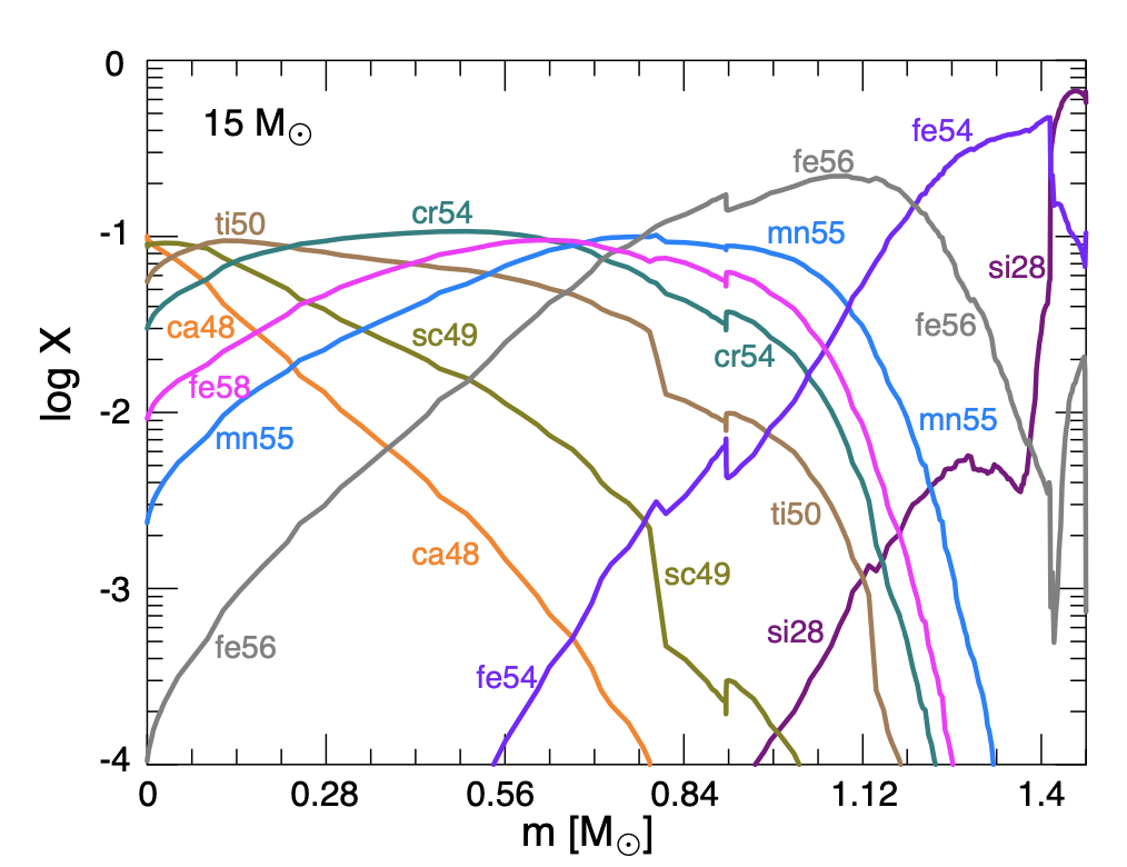
Finally, I thought I’d include a mass fraction’s plot, just because I have always enjoyed producing these when I ran models in MESA. I think they are some of the most interesting plots that can be generated, as they allow you to see in somewhat real time what is happening on an atomic level inside a star. This specific plot presents the mass fractions of the ten most abundant isotopes within an iron core at the onset of core collapse of a 15 M⊙ object.
Overall, I learned less about isochrones than I was hoping to, but got a great look into the more adult side of MESA — a side that would have frightened and intimidated me a year ago but one that I am incredibly excited an interested by today!