Blog Post #6

What I worked On This Week

Reduction pipeline updates

This week I performed what I believe to be the last few updates to my reduction pipeline that will be necessary for our project. The pipeline now automatically sorts the raw data from each night into a detailed folder structure that divides the images by object, time, and band, while reducing them and stacking them into groups of 6. I made some small revisions to my time sorting algorithm, and in the past few days added support for the handling of E/W images where the cluster has crossed the meridian. With those additions, I believe my reduction model is complete and pretty solid.

Since I have been working on colab for most of the semester, I took this past week to make the full change to a local processing system through jupyter notebooks. Thankfully, my code was able to port incredibly seamlessly, and after installing a few dependencies, the entire pipeline ran faster on my local machine than it did on the cloud. All the data is handled from an external solid state flash storage and all the code is backed up over the cloud. From here on out I should be running local!

Additional Nights of Data

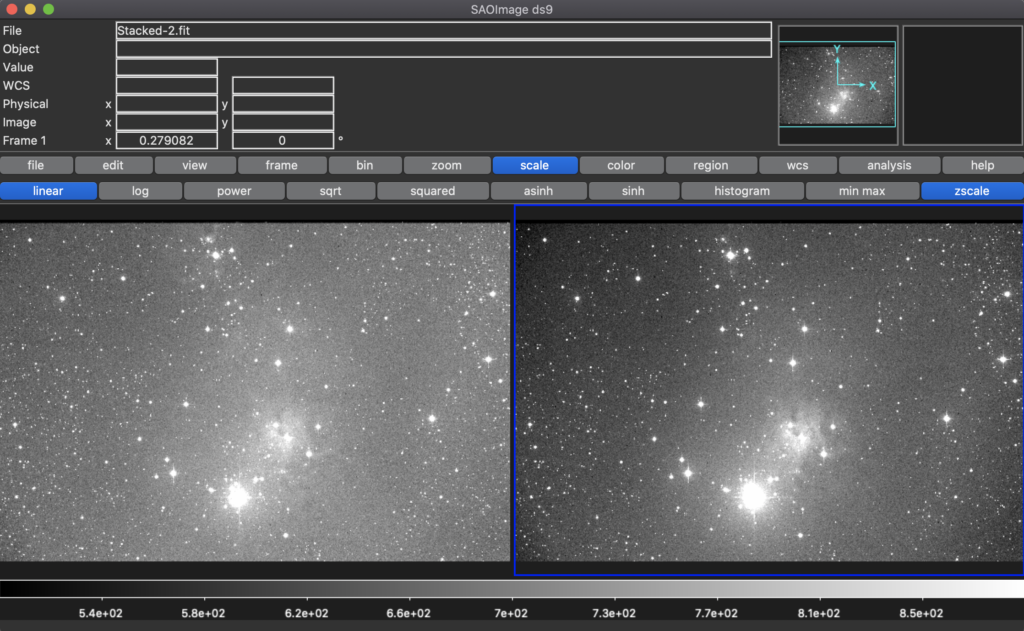
I had run multiple nights of data through my pipeline before, so this wasn’t really anything new. This was the first time, however, that I ran all nights at the same time and simply let the module take over. And it worked perfectly. I reduced our first seven nights of data and will continue to reduce the rest as I download it from the FTP server (my internet has been playing games with me over the past few days). Looking at the aligned images, I believe everything is going well. The last thing I might want to play with is exactly which image everything will be aligning against, but my code can take that in as a global input, and runs quickly enough that it will be very easy to swap out alignment images to compare and contrast the differences. (This is also a conversation I’m sure we’ll have as a group.)

Cross Comparison of Reduction Codes

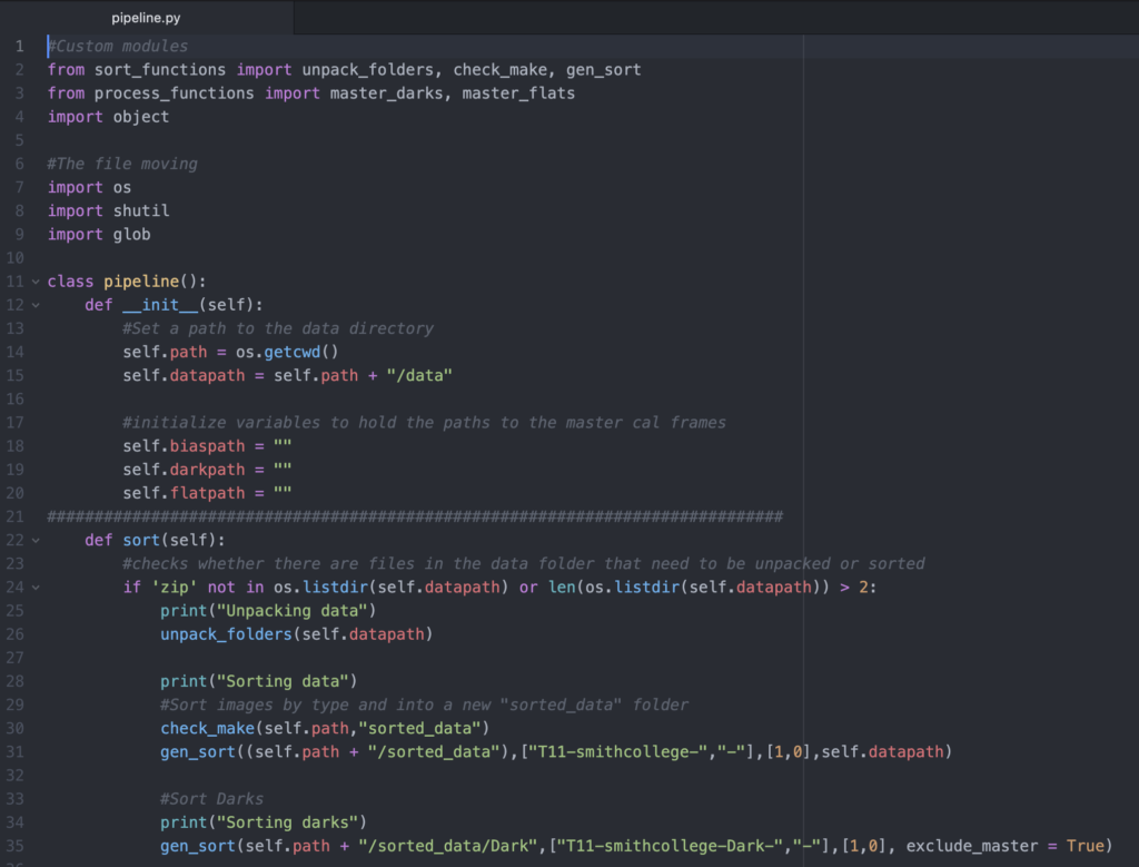
I focused on comparing my reduction pipeline code with Cat as we worked on the same final project last semester and have generally worked off of the same starting code base since then. I was very interested to see her approach from the code perspective as she has mentioned a few times that she took a very object oriented approach to the entire reduction process. Reading through her code, I was very impressed by the organization and simplicity with which her methods were laid out. From a top down view, her code is split into a number of modules and classes, which makes some of the processes much easier to follow. My pipeline is still mostly in one single module file and, while commented quite well – if i do say so myself 🙂 – it can be a bit tricky to follow the piecemeal structure that emerged from an entire semester of learning the reduction process.

I have so far this semester resisted the urge of dumping most if not all of my code from last semester and rewriting from scratch. I know that I could improve greatly on what I wrote back then and most likely reduce both the size and complexity of my module by a hug factor. That said, it works very well and I think it is probably for the best if I forget what is under the hood and simply look towards the next code, instead of fixing what isn’t really broken. With all of that said, much of Cat’s code is quite similar to mine. Our flat fielding and bias/dark subtracting functions have both been altered from last semester to include for fine precision control, while many of our base functions such as median combination and low level sorting algorithms haven’t been altered from the labs where they were introduced.

Our main differences are in the algorithms we have implemented recently to sort and catalogue our new data. Cat made use of a fantastic object oriented approach which allows for reduction directly from the command line. While her code is not extremely commented yet, it is relatively easy to understand and follow the logic she employs in her calculations. We will have to discuss as a group how we want our final sorting algorithms to run and whether or not we all really want them to be object oriented (personally I have no qualms as long as we all understand the code and what it is attempting to do). Altogether it was a ton of fun to get to see a new and different approach to the same project we’ve all been working on!

Astrometry.net

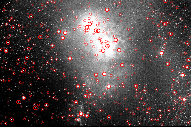
I used astrometry.net like we did in class to accurately locate the section of sky we are imaging and eventually to source the stars in our cluster, separating them from field or background stars that could otherwise add error to our calculations. Below is an image from these calculations identifying the stars that astrometry.net resolved in and around the cluster. I am still in the process of fully separating the NGC 2264 stars from the rest in the manner we discussed a couple classes back, but I plan to make sizable progress on that front this week.

GM Aur activity

My partner in this was Cat Sarosi. We worked on these answers during and after class in a single document, and contributed equally to the work below.

What do each of the weight matrices represent?

• w1: Tracks which exposures (rows) should be excluded as a whole from the solution (across all stars). Type: boolean
• w2: Tracks which stars (columns) should be excluded as a whole from the solution (across all exposures). Type: boolean
• w3: Tracks which stars (indices) should be excluded specifically from the solution. Type: boolean
• w4: The weights for each star-exposure pair in the array, where the weight is based on an error estimate from the CCD equation. Type: float
• . Type:  float #Instrumental magnitude array

What does “basicExclude” do to the weight matrix? Why is this a necessary step?

• Commenting it out results in an error due to the presence of nans/infinities, so it appears to unweight (remove) observations containing nans/infinities. Observation of the source code reveals that it removes a star from a specific exposure if it contains nans or infinities, or if it is below the snr ratio. It also tracks stars that do not appear in any exposure or exposures that do not contain any stars

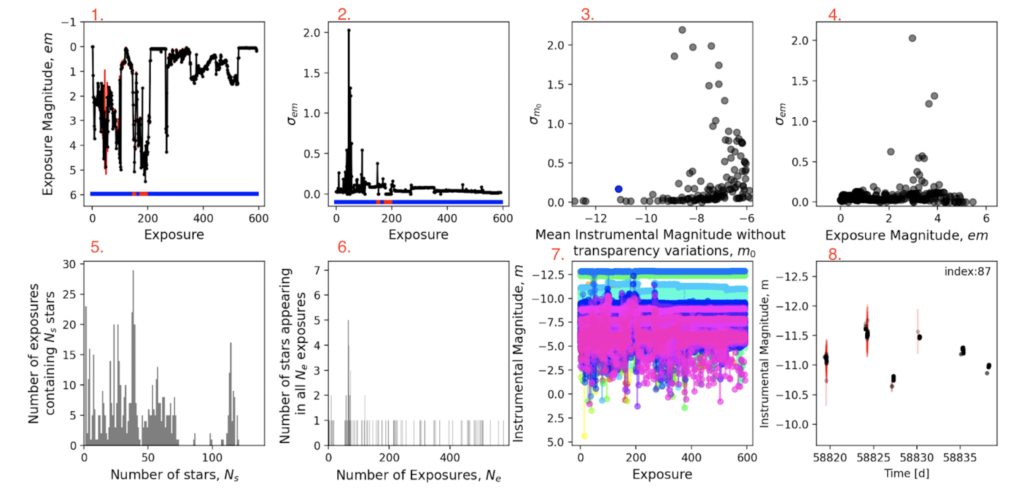
• Panel 1: Exposure number v. exposure magnitude (em)
• Panel 2: Exposure number v. the standard deviation in exposure magnitude em
• Panel 3: Mean instrumental magnitude m₀ (without transparency variations)
• Panel 4: Exposure magnitude (em) v. standard deviation in exposure magnitude em
• Panel 5: Number of stars (N_S) v. Number of exposures containing N_S stars
• Panel 6: Number of exposures (N_e) v. Number of stars appearing in all N_e exposures
• Panel 7: Exposure number v. Instrumental Magnitude (m)
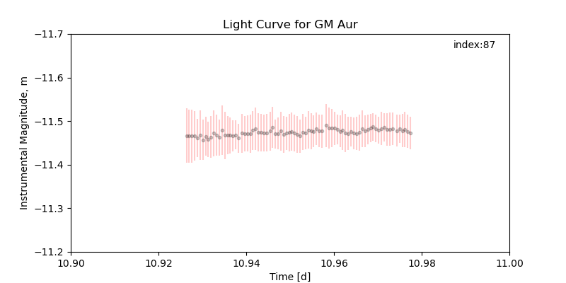
• Panel 8: Time (d) v. Instrumental Magnitude (m) for the object with the index 87 

Which panels can we use to identify variable stars? 

• Panel 3, shows what stars have a large standard deviations on their instrument magnitude  m₀ 
• Panel 8, shows a light curve for a given star 
• Panel 7, theoretically, if there weren’t so many objects displayed in it

What sort of stars make good comparison objects? Which ones make bad ones?

• Stars that have a low standard deviation on m₀  and appear in multiple exposures. Bad comparison objects are stars that only appear in one exposure or stars with a high standard deviation on m₀ indicating that they might be variable stars (this can be confirmed by looking at the light curve)

What sort of SNR cutoff seems to be good for this dataset?

• An SNR cutoff of about 5 seems to be good for this dataset. It removes enough stars to minimize the noise but not too many that we lose any noticeable information about the behavior of the light curve over time.

How should we decide which stars are excluded from the solution?

• Stars with a low SNR and stars with a high magnitude deviation should be excluded from our calculations. The more noisy our estimates are for stellar magnitudes and the more variable a star’s brightness is, the more we want to exclude it from the solution. 

How should we decide which exposures are excluded from the solution?

• Exposures that only have a few resolvable stars and exposures that have very high standard deviations should be excluded from the solution as they most likely had some sort of large atmospheric or statistically significant interference and could introduce unnecessary error into our photometric calculations.

How does the solver navigate around all-zero weights in columns/rows of the weight matrix? Why is this a necessary step?

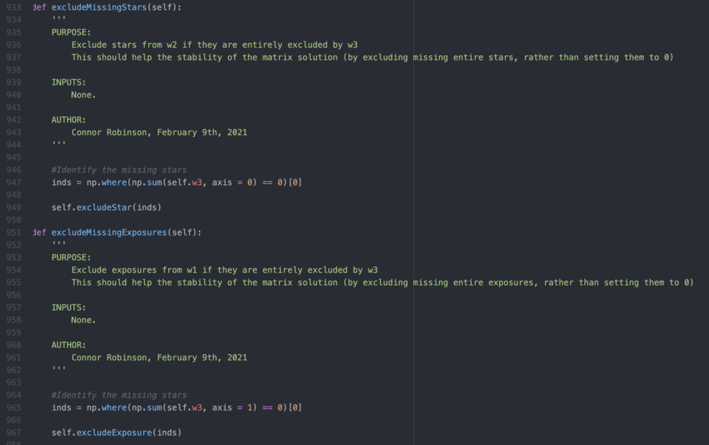
• If either stars or entire exposures are completely nullified by the weight matrix, the solver chooses to exclude them entirely instead of just setting their values to zero. This greatly reduces the load on the solver in its calculations, thereby increasing the runtime efficiency of the program as a whole while increasing its overall performance.

Are there differences between this dataset and your dataset? How will you approach these differences?

• Our dataset spans multiple bands, and we will be considering the light curve of more than just one object of interest. I assume we will need to be sure that we make similar decisions across bands in order to keep results consistent. In addition, our dataset will have many more nights of observing, with many fewer observations each night. This means the light curves will be spread out over a much larger time frame but will not provide as much information about variation on short times scales.

What are the benefits of doing this in an interactive manner?

• An interactive approach to this sort of calculation allows us to very easily determine what data points we want to include and exclude on the fly. Since we will be relying quite a bit on our own intuition to make the judgment about which data points to throw out, and interactive interface allows immediate feedback to these choices, greatly increasing the efficiency of the process. (Thank you Connor!) 

Mist Isochrone Paper

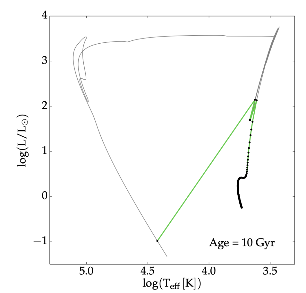
This week I chose to discuss the paper that introduced the MIST isochrones. The paper essentially focuses on using the stellar evolution code MESA to generate simulations of young and evolving stars. It then calculates probabilistic paths for stars of different initial masses, and then uses extremely clever interpolation models to generate isochrones for an effectively continuous range of initial masses. Shown below is a diagram from the paper that compares a MIST isochrone to an earlier isochrone model that generates from a much lower level set of calculations.

They also discussed quite a bit of evolutionary modeling theory. In the figure below, they are comparing EEPs or Equivalent Evolutionary Tracks which they define as “a series of points that can be identified in all stellar evolution tracks.” The paper goes on to discuss the use of EEPs and the eventual generation of isochrones. I am still working through some of the more technical theory, and hope to present all that I have learned in class.

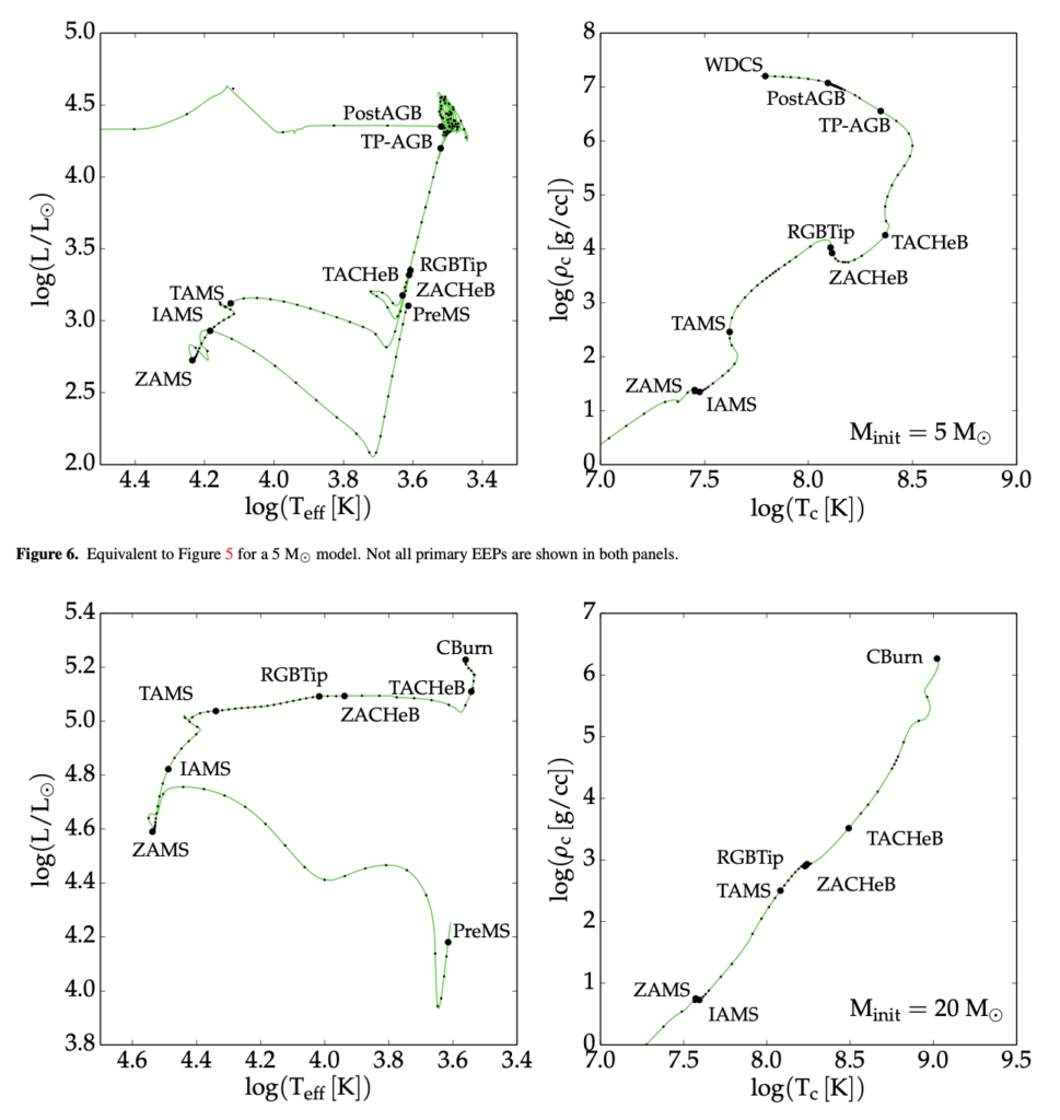
The overall concept of the paper is relatively technical, but outlines the improvements and deficiencies of the MIST models, as of 2016. This will be very helpful if we want to use their isochrone models, or possibly even recreate some of their findings in MESA ourselves. I’ll have some more graphics and quite a bit more to say in class tomorrow!