Introduction
Well, it’s been another week hasn’t it. Wow time really is flying. My resolution for next week is to start writing these earlier. I’ve been quite good at spacing out the workload across a number of days, but somehow the writing always ends up happening the night of. Anywho, on to what I’ve been up to. (I also can’t wait to see how these start to get less and less formal as the semester continues. I aspire to some of the stories Khalid has told me about past blogs.)
I spent the most time this week writing code to handle the iTelescope data better than what I was doing before. I had been manually unzipping files and dropping them into the drive, which just isn’t a good way to live. I cleaned up the process with some new packages and a bit of recursion, so that now unpacking new data should be fantastically convenient. I learned last semester that a bit of organizational preparation pays off so much later down the line.
Data Reduction
Part 1 – the struggle
I began this week by going through my old code for bias and dark subtracting, just to make sure I understood everything that was going on then and now. It was pretty well written and commented, so the review wasn’t too bad. The fun started when I began to look into the flats.
As a review for those reading this in the far future, our bias frames from iTelescope are somehow skewed to much higher counts than they should be reading, thus we have elected to not use them in our reduction pipeline. Instead, we will use un-bias-subtracted master darks, which when removed from our own data, should account for some of the bias frame reduction themselves. We will then estimate read noise separately from the standard deviation of the biases — I believe we can still trust the bias distribution because we are assuming a linear offset somewhere in the bias-taking process — and be left will well reduced images.
The flats, imaged by iTelescope around a year ago, are not ideal to say the least. I began by making the wonderfully clever decision to attempt to generate my own master flats instead of settling for the master flats already provided. I spent a good few hours preparing them for reduction and tweaking my pipeline to correctly handle the zipped files and new folder structure. I also had to generalize my code to handle more bands, all of which went well. The issues I ran into, however, are as follows.
First, the exposure times for the flats are all over the place. It appears as there was no set exposure length used, as all the flats from the most recent flat-taking comprised over 180 unique exposure times. Now this wouldn’t normally be an issue, as we could just scale our bias-subtracted darks to match the exposure time of the flats. But we can’t scale our bias-subtracted darks, because we don’t have them. If we were to scale our darks without bias subtracting, we would be scaling the bias counts as well, thereby skewing our eventual photometry.
As I was looking into this, I found a second, interesting problem. The flat frames as given include in their headers that they are already bias subtracted. I found this confusing for a number of reasons, first and foremost because I can only imagine the bias frames they used are just as skewed as ours. Secondly, it means that even if they used good bias data to reduce the flats, we couldn’t subtract off our darks without double correcting for bias. Sigh — at least I only spent most of the weekend on this
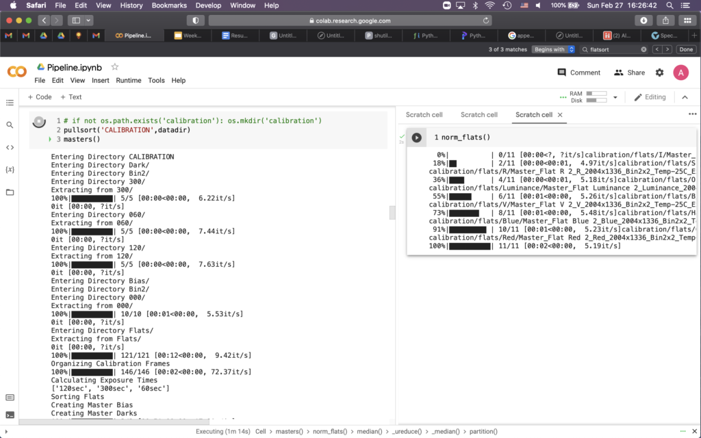
Part 2 – master flats
So I ended up grabbing the master flats already given to us by iTelescope. I’m pretty sure they also only say that they have been bias subtracted and make no mention of dark correction, but I am not completely sure. It appears that there are a few occurrences of hot pixels that would be correctable with good dark subtraction, but alas, the problems referenced above might preclude us from that. Also, them being master flats and all, shouldn’t they already be dark corrected? Problems for this coming week, I guess.
And that’s where I am. I flat fielded a few science images by hand (i.e. not through my pipeline) but I had yet to normalize the master flats so they turned out pretty weirdly. Once I figure out what to do about the flats, I should be able to rely on my 337 pipeline pretty heavily for the final reduction steps and for photometry, so that’s the plan for next week. I’ll have to generalize a bit to allow data from multiple nights to be processed at once. Writing that though, I’m not even sure that will be necessary. It would honestly be more convenient to process each night separately one by one, leaving my code relatively solid for what we’ll eventually need. That leaves next steps to be photometry calculations and final tweaks to the flat fielding of science images.
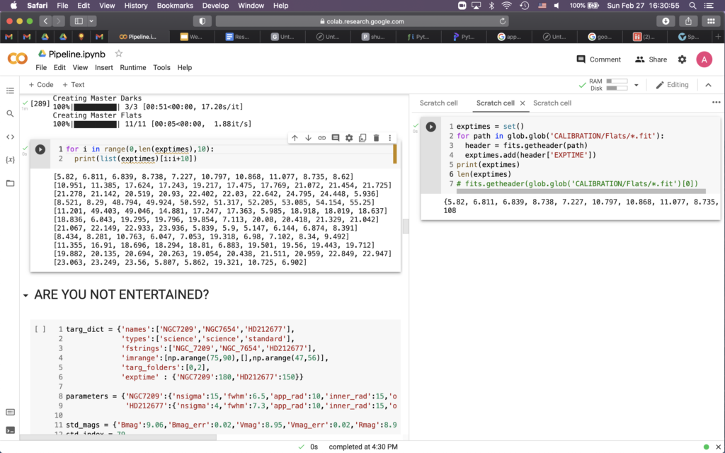
Part 3 – gain estimation
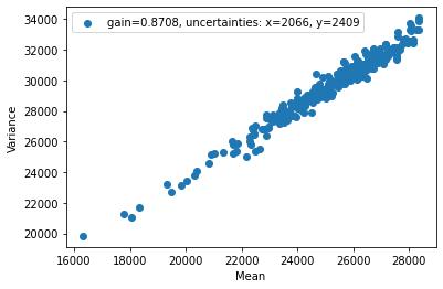
I don’t think I need to say a lot about this as we discussed the process quite a bit in class. We estimate the gain of the telescope by using two flats and a bit of math. The equations we derived in class allow us to write some code to determine a linear relation between the variance and the mean of the flats. The slope of the line of best fit will then give us an estimate for the gain of the telescope. I personally calculated a gain of 0.871 which seemed to be in line with what the rest of class determined.
My Paper
The paper that I chose to cover is Bastian et al. 2010. It’s a review paper covering initial mass functions, their development, and their applications. Overall, it’s a 40 page paper that covers much more information than will be necessary or useful to our project. I chose it though because it will serve to give me some background on the science behind our project. I have never had a course in galactic astronomy, and currently am a bit behind on the nomenclature and intuition that my project partners possess. And I should say that I don’t mind the disadvantage on bit — it just means I have more to learn. And I think that’s always a good thing.
I have focused mostly on the first few sections of my paper, as they give an introduction to the ideas surrounding a determination of an IMF. The paper gives a brief history of different power laws thought to represent mass functions as different mass regimes. It then introduces the idea that a split power law is the most likely distribution, leaving the Saltpeter relation for the high mass stellar regime. From the 1960s onward, there have been a large number of proposed IMFs, each with varying degrees of community acceptance. The three most important Saltpeter, Kroupa, and Chabrier. The paper refers to IMFs with a slope of Γ = 1.35 as having a Saltpeter slope, while it refers to segmented IMFs with a differing slope for lower mass stars as Kroupa IMFs.
Bastian goes on to discuss the observational challenges inherent in documenting IMFs. The assumption of both temporal and spacial uniformity seems to be essential in accurately estimating an IMF, yet we are unsure if these assumptions hold true. It is also important to consider multiplicity in IMF measurements, as binary systems can skew documented brightnesses and allow observers to miss low mass stars completely.
In addition, Bastian mentions regular and rampant confusion in the literature about slope conventions, uncertainties, and core equations to describing IMFs. Many papers don’t include uncertainties in their slope estimations, while many end up estimating slopes for entirely different equations with different numbers of free parameters. Even though more free parameters should lead to better scientific results, it is unclear many times if the relations between the free parameters is even physically significant at all.
Bastian goes on to discuss the utility of the IMF and attempts to give justification to the necessity of observations and estimates of the function. As this paper is a review paper, I’ll suffice with the summaries given above. I can go into more detail about the later sections of the paper, but what I have written above seems to be the most relevant background to our project. I have included three relavant figures from the paper below.
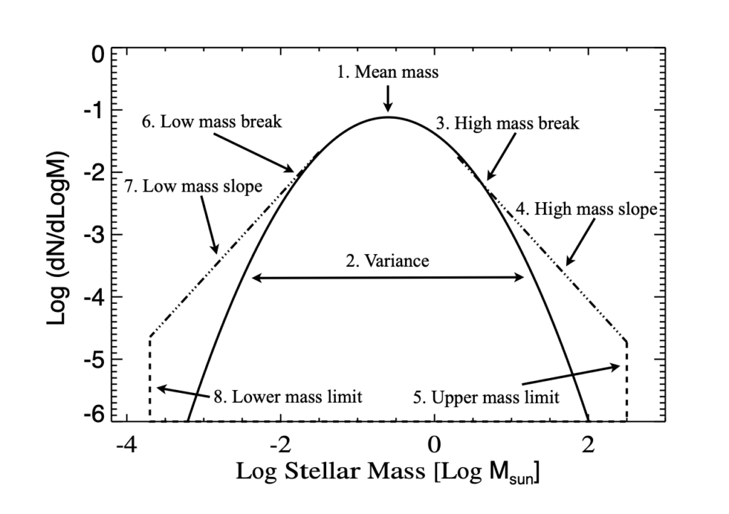
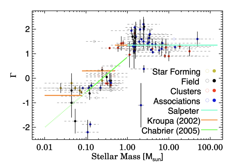
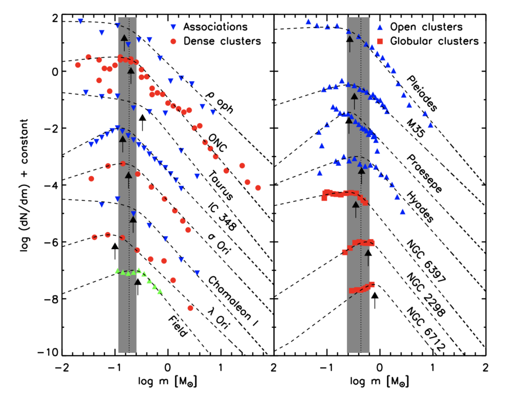
The derived mass function of young star-forming regions. Plots like this are good for me to get used to as we might end up generating similar slopes and curves as the ones seen here. The more I read from this paper the more clearly I understand the scope of our project. 🙂